Streaming
Calcite has extended SQL and relational algebra in order to support streaming queries.
- Introduction
- An example schema
- A simple query
- Filtering rows
- Projecting expressions
- Tumbling windows
- Tumbling windows, improved
- Hopping windows
- GROUPING SETS
- Filtering after aggregation
- Sub-queries, views and SQL’s closure property
- Converting between streams and relations
- The “pie chart” problem: Relational queries on streams
- Sorting
- Table constructor
- Sliding windows
- Cascading windows
- Joining streams to tables
- Joining streams to streams
- DML
- Punctuation
- State of the stream
- Functions
- References
Introduction
Streams are collections to records that flow continuously, and forever. Unlike tables, they are not typically stored on disk, but flow over the network and are held for short periods of time in memory.
Streams complement tables because they represent what is happening in the present and future of the enterprise whereas tables represent the past. It is very common for a stream to be archived into a table.
Like tables, you often want to query streams in a high-level language based on relational algebra, validated according to a schema, and optimized to take advantage of available resources and algorithms.
Calcite’s SQL is an extension to standard SQL, not another ‘SQL-like’ language. The distinction is important, for several reasons:
- Streaming SQL is easy to learn for anyone who knows regular SQL.
- The semantics are clear, because we aim to produce the same results on a stream as if the same data were in a table.
- You can write queries that combine streams and tables (or the history of a stream, which is basically an in-memory table).
- Lots of existing tools can generate standard SQL.
If you don’t use the STREAM keyword, you are back in regular
standard SQL.
An example schema
Our streaming SQL examples use the following schema:
-
Orders (rowtime, productId, orderId, units)- a stream and a table -
Products (rowtime, productId, name)- a table -
Shipments (rowtime, orderId)- a stream
A simple query
Let’s start with the simplest streaming query:
SELECT STREAM *
FROM Orders;

  rowtime | productId | orderId | units
----------+-----------+---------+-------
 10:17:00 |        30 |       5 |     4
 10:17:05 |        10 |       6 |     1
 10:18:05 |        20 |       7 |     2
 10:18:07 |        30 |       8 |    20
 11:02:00 |        10 |       9 |     6
 11:04:00 |        10 |      10 |     1
 11:09:30 |        40 |      11 |    12
 11:24:11 |        10 |      12 |     4
This query reads all columns and rows from the Orders stream.
Like any streaming query, it never terminates. It outputs a record whenever
a record arrives in Orders.
Type Control-C to terminate the query.
The STREAM keyword is the main extension in streaming SQL. It tells the
system that you are interested in incoming orders, not existing ones. The query
SELECT *
FROM Orders;

  rowtime | productId | orderId | units
----------+-----------+---------+-------
 08:30:00 |        10 |       1 |     3
 08:45:10 |        20 |       2 |     1
 09:12:21 |        10 |       3 |    10
 09:27:44 |        30 |       4 |     2

4 records returned.
is also valid, but will print out all existing orders and then terminate. We call it a relational query, as opposed to streaming. It has traditional SQL semantics.
Orders is special, in that it has both a stream and a table. If you try to run
a streaming query on a table, or a relational query on a stream, Calcite gives
an error:
SELECT * FROM Shipments;

ERROR: Cannot convert stream 'SHIPMENTS' to a table

SELECT STREAM * FROM Products;

ERROR: Cannot convert table 'PRODUCTS' to a stream
Filtering rows
Just as in regular SQL, you use a WHERE clause to filter rows:
SELECT STREAM *
FROM Orders
WHERE units > 3;

  rowtime | productId | orderId | units
----------+-----------+---------+-------
 10:17:00 |        30 |       5 |     4
 10:18:07 |        30 |       8 |    20
 11:02:00 |        10 |       9 |     6
 11:09:30 |        40 |      11 |    12
 11:24:11 |        10 |      12 |     4
Projecting expressions
Use expressions in the SELECT clause to choose which columns to return or
compute expressions:
SELECT STREAM rowtime,
  'An order for ' || units || ' '
    || CASE units WHEN 1 THEN 'unit' ELSE 'units' END
    || ' of product #' || productId AS description
FROM Orders;

  rowtime | description
----------+---------------------------------------
 10:17:00 | An order for 4 units of product #30
 10:17:05 | An order for 1 unit of product #10
 10:18:05 | An order for 2 units of product #20
 10:18:07 | An order for 20 units of product #30
 11:02:00 | An order by 6 units of product #10
 11:04:00 | An order by 1 unit of product #10
 11:09:30 | An order for 12 units of product #40
 11:24:11 | An order by 4 units of product #10
We recommend that you always include the rowtime column in the SELECT
clause. Having a sorted timestamp in each stream and streaming query makes it
possible to do advanced calculations later, such as GROUP BY and JOIN.
Tumbling windows
There are several ways to compute aggregate functions on streams. The differences are:
- How many rows come out for each row in?
- Does each incoming value appear in one total, or more?
- What defines the “window”, the set of rows that contribute to a given output row?
- Is the result a stream or a relation?
There are various window types:
- tumbling window (GROUP BY)
- hopping window (multi GROUP BY)
- sliding window (window functions)
- cascading window (window functions)
and the following diagram shows the kinds of query in which to use them:
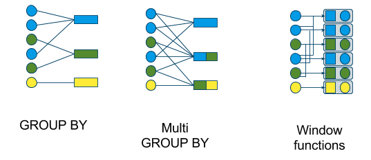
First we’ll look a tumbling window, which is defined by a streaming
GROUP BY. Here is an example:
SELECT STREAM CEIL(rowtime TO HOUR) AS rowtime,
  productId,
  COUNT(*) AS c,
  SUM(units) AS units
FROM Orders
GROUP BY CEIL(rowtime TO HOUR), productId;

  rowtime | productId |       c | units
----------+-----------+---------+-------
 11:00:00 |        30 |       2 |    24
 11:00:00 |        10 |       1 |     1
 11:00:00 |        20 |       1 |     7
 12:00:00 |        10 |       3 |    11
 12:00:00 |        40 |       1 |    12
The result is a stream. At 11 o’clock, Calcite emits a sub-total for every
productId that had an order since 10 o’clock, timestamped 11 o’clock.
At 12 o’clock, it will emit
the orders that occurred between 11:00 and 12:00. Each input row contributes to
only one output row.
How did Calcite know that the 10:00:00 sub-totals were complete at 11:00:00,
so that it could emit them? It knows that rowtime is increasing, and it knows
that CEIL(rowtime TO HOUR) is also increasing. So, once it has seen a row
at or after 11:00:00, it will never see a row that will contribute to a 10:00:00
total.
A column or expression that is increasing or decreasing is said to be monotonic.
If column or expression has values that are slightly out of order, and the stream has a mechanism (such as punctuation or watermarks) to declare that a particular value will never be seen again, then the column or expression is said to be quasi-monotonic.
Without a monotonic or quasi-monotonic expression in the GROUP BY clause,
Calcite is
not able to make progress, and it will not allow the query:
SELECT STREAM productId,
  COUNT(*) AS c,
  SUM(units) AS units
FROM Orders
GROUP BY productId;

ERROR: Streaming aggregation requires at least one monotonic expression in GROUP BY clause
Monotonic and quasi-monotonic columns need to be declared in the schema.
The monotonicity is
enforced when records enter the stream and assumed by queries that read from
that stream. We recommend that you give each stream a timestamp column called
rowtime, but you can declare others to be monotonic, orderId, for example.
We discuss punctuation, watermarks, and other ways of making progress below.
Tumbling windows, improved
The previous example of tumbling windows was easy to write because the window
was one hour. For intervals that are not a whole time unit, say 2 hours or
2 hours and 17 minutes, you cannot use CEIL, and the expression gets more
complicated.
Calcite supports an alternative syntax for tumbling windows:
SELECT STREAM TUMBLE_END(rowtime, INTERVAL '1' HOUR) AS rowtime,
  productId,
  COUNT(*) AS c,
  SUM(units) AS units
FROM Orders
GROUP BY TUMBLE(rowtime, INTERVAL '1' HOUR), productId;

  rowtime | productId |       c | units
----------+-----------+---------+-------
 11:00:00 |        30 |       2 |    24
 11:00:00 |        10 |       1 |     1
 11:00:00 |        20 |       1 |     7
 12:00:00 |        10 |       3 |    11
 12:00:00 |        40 |       1 |    12
As you can see, it returns the same results as the previous query. The TUMBLE
function returns a grouping key that is the same for all the rows that will end
up in a given summary row; the TUMBLE_END function takes the same arguments
and returns the time at which that window ends;
there is also a TUMBLE_START function.
TUMBLE has an optional parameter to align the window.
In the following example,
we use a 30 minute interval and 0:12 as the alignment time,
so the query emits summaries at 12 and 42 minutes past each hour:
SELECT STREAM
  TUMBLE_END(rowtime, INTERVAL '30' MINUTE, TIME '0:12') AS rowtime,
  productId,
  COUNT(*) AS c,
  SUM(units) AS units
FROM Orders
GROUP BY TUMBLE(rowtime, INTERVAL '30' MINUTE, TIME '0:12'),
  productId;

  rowtime | productId |       c | units
----------+-----------+---------+-------
 10:42:00 |        30 |       2 |    24
 10:42:00 |        10 |       1 |     1
 10:42:00 |        20 |       1 |     7
 11:12:00 |        10 |       2 |     7
 11:12:00 |        40 |       1 |    12
 11:42:00 |        10 |       1 |     4
Hopping windows
Hopping windows are a generalization of tumbling windows that allow data to be kept in a window for a longer than the emit interval.
For example, the following query emits a row timestamped 11:00 containing data from 08:00 to 11:00 (or 10:59.9 if we’re being pedantic), and a row timestamped 12:00 containing data from 09:00 to 12:00.
SELECT STREAM
  HOP_END(rowtime, INTERVAL '1' HOUR, INTERVAL '3' HOUR) AS rowtime,
  COUNT(*) AS c,
  SUM(units) AS units
FROM Orders
GROUP BY HOP(rowtime, INTERVAL '1' HOUR, INTERVAL '3' HOUR);

  rowtime |        c | units
----------+----------+-------
 11:00:00 |        4 |    27
 12:00:00 |        8 |    50
In this query, because the retain period is 3 times the emit period, every input
row contributes to exactly 3 output rows. Imagine that the HOP function
generates a collection of group keys for incoming row, and places its values
in the accumulators of each of those group keys. For example,
HOP(10:18:00, INTERVAL '1' HOUR, INTERVAL '3') generates 3 periods
[08:00, 09:00)
[09:00, 10:00)
[10:00, 11:00)
This raises the possibility of allowing user-defined partitioning functions
for users who are not happy with the built-in functions HOP and TUMBLE.
We can build complex complex expressions such as an exponentially decaying moving average:
SELECT STREAM HOP_END(rowtime),
  productId,
  SUM(unitPrice * EXP((rowtime - HOP_START(rowtime)) SECOND / INTERVAL '1' HOUR))
   / SUM(EXP((rowtime - HOP_START(rowtime)) SECOND / INTERVAL '1' HOUR))
FROM Orders
GROUP BY HOP(rowtime, INTERVAL '1' SECOND, INTERVAL '1' HOUR),
  productId
Emits:
- a row at
11:00:00containing rows in[10:00:00, 11:00:00); - a row at
11:00:01containing rows in[10:00:01, 11:00:01).
The expression weighs recent orders more heavily than older orders. Extending the window from 1 hour to 2 hours or 1 year would have virtually no effect on the accuracy of the result (but use more memory and compute).
Note that we use HOP_START inside an aggregate function (SUM) because it
is a value that is constant for all rows within a sub-total. This
would not be allowed for typical aggregate functions (SUM, COUNT
etc.).
If you are familiar with GROUPING SETS, you may notice that partitioning
functions can be seen as a generalization of GROUPING SETS, in that they
allow an input row to contribute to multiple sub-totals.
The auxiliary functions for GROUPING SETS,
such as GROUPING() and GROUP_ID,
can be used inside aggregate functions, so it is not surprising that
HOP_START and HOP_END can be used in the same way.
GROUPING SETS
GROUPING SETS is valid for a streaming query provided that every
grouping set contains a monotonic or quasi-monotonic expression.
CUBE and ROLLUP are not valid for streaming query, because they will
produce at least one grouping set that aggregates everything (like
GROUP BY ()).
Filtering after aggregation
As in standard SQL, you can apply a HAVING clause to filter rows emitted by
a streaming GROUP BY:
SELECT STREAM TUMBLE_END(rowtime, INTERVAL '1' HOUR) AS rowtime,
  productId
FROM Orders
GROUP BY TUMBLE(rowtime, INTERVAL '1' HOUR), productId
HAVING COUNT(*) > 2 OR SUM(units) > 10;

  rowtime | productId
----------+-----------
 10:00:00 |        30
 11:00:00 |        10
 11:00:00 |        40
Sub-queries, views and SQL’s closure property
The previous HAVING query can be expressed using a WHERE clause on a
sub-query:
SELECT STREAM rowtime, productId
FROM (
  SELECT TUMBLE_END(rowtime, INTERVAL '1' HOUR) AS rowtime,
    productId,
    COUNT(*) AS c,
    SUM(units) AS su
  FROM Orders
  GROUP BY TUMBLE(rowtime, INTERVAL '1' HOUR), productId)
WHERE c > 2 OR su > 10;

  rowtime | productId
----------+-----------
 10:00:00 |        30
 11:00:00 |        10
 11:00:00 |        40
HAVING was introduced in the early days of SQL, when a way was needed to
perform a filter after aggregation. (Recall that WHERE filters rows before
they enter the GROUP BY clause.)
Since then, SQL has become a mathematically closed language, which means that any operation you can perform on a table can also perform on a query.
The closure property of SQL is extremely powerful. Not only does it render
HAVING obsolete (or, at least, reduce it to syntactic sugar), it makes views
possible:
CREATE VIEW HourlyOrderTotals (rowtime, productId, c, su) AS
  SELECT TUMBLE_END(rowtime, INTERVAL '1' HOUR),
    productId,
    COUNT(*),
    SUM(units)
  FROM Orders
  GROUP BY TUMBLE(rowtime, INTERVAL '1' HOUR), productId;

SELECT STREAM rowtime, productId
FROM HourlyOrderTotals
WHERE c > 2 OR su > 10;

  rowtime | productId
----------+-----------
 10:00:00 |        30
 11:00:00 |        10
 11:00:00 |        40
Sub-queries in the FROM clause are sometimes referred to as “inline views”,
but really, they are more fundamental than views. Views are just a convenient
way to carve your SQL into manageable chunks by giving the pieces names and
storing them in the metadata repository.
Many people find that nested queries and views are even more useful on streams than they are on relations. Streaming queries are pipelines of operators all running continuously, and often those pipelines get quite long. Nested queries and views help to express and manage those pipelines.
And, by the way, a WITH clause can accomplish the same as a sub-query or
a view:
WITH HourlyOrderTotals (rowtime, productId, c, su) AS (
  SELECT TUMBLE_END(rowtime, INTERVAL '1' HOUR),
    productId,
    COUNT(*),
    SUM(units)
  FROM Orders
  GROUP BY TUMBLE(rowtime, INTERVAL '1' HOUR), productId)
SELECT STREAM rowtime, productId
FROM HourlyOrderTotals
WHERE c > 2 OR su > 10;

  rowtime | productId
----------+-----------
 10:00:00 |        30
 11:00:00 |        10
 11:00:00 |        40
Converting between streams and relations
Look back at the definition of the HourlyOrderTotals view.
Is the view a stream or a relation?
It does not contain the STREAM keyword, so it is a relation.
However, it is a relation that can be converted into a stream.
You can use it in both relational and streaming queries:
# A relation; will query the historic Orders table.
# Returns the largest number of product #10 ever sold in one hour.
SELECT max(su)
FROM HourlyOrderTotals
WHERE productId = 10;

# A stream; will query the Orders stream.
# Returns every hour in which at least one product #10 was sold.
SELECT STREAM rowtime
FROM HourlyOrderTotals
WHERE productId = 10;
This approach is not limited to views and sub-queries.
Following the approach set out in CQL [1], every query
in streaming SQL is defined as a relational query and converted to a stream
using the STREAM keyword in the top-most SELECT.
If the STREAM keyword is present in sub-queries or view definitions, it has no
effect.
At query preparation time, Calcite figures out whether the relations referenced in the query can be converted to streams or historical relations.
Sometimes a stream makes available some of its history (say the last 24 hours of data in an Apache Kafka [2] topic) but not all. At run time, Calcite figures out whether there is sufficient history to run the query, and if not, gives an error.
The “pie chart” problem: Relational queries on streams
One particular case where you need to convert a stream to a relation occurs in what I call the “pie chart problem”. Imagine that you need to write a web page with a chart, like the following, that summarizes the number of orders for each product over the last hour.
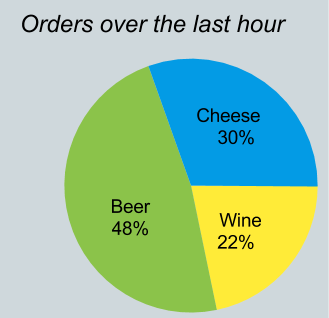
But the Orders stream only contains a few records, not an hour’s summary.
We need to run a relational query on the history of the stream:
SELECT productId, count(*)
FROM Orders
WHERE rowtime BETWEEN current_timestamp - INTERVAL '1' HOUR
              AND current_timestamp;
If the history of the Orders stream is being spooled to the Orders table,
we can answer the query, albeit at a high cost. Better, if we can tell the
system to materialize one hour summary into a table,
maintain it continuously as the stream flows,
and automatically rewrite queries to use the table.
Sorting
The story for ORDER BY is similar to GROUP BY.
The syntax looks like regular SQL, but Calcite must be sure that it can deliver
timely results. It therefore requires a monotonic expression on the leading edge
of your ORDER BY key.
SELECT STREAM CEIL(rowtime TO hour) AS rowtime, productId, orderId, units
FROM Orders
ORDER BY CEIL(rowtime TO hour) ASC, units DESC;

  rowtime | productId | orderId | units
----------+-----------+---------+-------
 10:00:00 |        30 |       8 |    20
 10:00:00 |        30 |       5 |     4
 10:00:00 |        20 |       7 |     2
 10:00:00 |        10 |       6 |     1
 11:00:00 |        40 |      11 |    12
 11:00:00 |        10 |       9 |     6
 11:00:00 |        10 |      12 |     4
 11:00:00 |        10 |      10 |     1
Most queries will return results in the order that they were inserted, because the engine is using streaming algorithms, but you should not rely on it. For example, consider this:
SELECT STREAM *
FROM Orders
WHERE productId = 10
UNION ALL
SELECT STREAM *
FROM Orders
WHERE productId = 30;

  rowtime | productId | orderId | units
----------+-----------+---------+-------
 10:17:05 |        10 |       6 |     1
 10:17:00 |        30 |       5 |     4
 10:18:07 |        30 |       8 |    20
 11:02:00 |        10 |       9 |     6
 11:04:00 |        10 |      10 |     1
 11:24:11 |        10 |      12 |     4
The rows with productId = 30 are apparently out of order, probably because
the Orders stream was partitioned on productId and the partitioned streams
sent their data at different times.
If you require a particular ordering, add an explicit ORDER BY:
SELECT STREAM *
FROM Orders
WHERE productId = 10
UNION ALL
SELECT STREAM *
FROM Orders
WHERE productId = 30
ORDER BY rowtime;

  rowtime | productId | orderId | units
----------+-----------+---------+-------
 10:17:00 |        30 |       5 |     4
 10:17:05 |        10 |       6 |     1
 10:18:07 |        30 |       8 |    20
 11:02:00 |        10 |       9 |     6
 11:04:00 |        10 |      10 |     1
 11:24:11 |        10 |      12 |     4
Calcite will probably implement the UNION ALL by merging using rowtime,
which is only slightly less efficient.
You only need to add an ORDER BY to the outermost query. If you need to,
say, perform GROUP BY after a UNION ALL, Calcite will add an ORDER BY
implicitly, in order to make the GROUP BY algorithm possible.
Table constructor
The VALUES clause creates an inline table with a given set of rows.
Streaming is disallowed. The set of rows never changes, and therefore a stream would never return any rows.
> SELECT STREAM * FROM (VALUES (1, 'abc'));

ERROR: Cannot stream VALUES
Sliding windows
Standard SQL features so-called “analytic functions” that can be used in the
SELECT clause. Unlike GROUP BY, these do not collapse records. For each
record that goes in, one record comes out. But the aggregate function is based
on a window of many rows.
Let’s look at an example.
SELECT STREAM rowtime,
  productId,
  units,
  SUM(units) OVER (ORDER BY rowtime RANGE INTERVAL '1' HOUR PRECEDING) unitsLastHour
FROM Orders;
The feature packs a lot of power with little effort. You can have multiple
functions in the SELECT clause, based on multiple window specifications.
The following example returns orders whose average order size over the last 10 minutes is greater than the average order size for the last week.
SELECT STREAM *
FROM (
  SELECT STREAM rowtime,
    productId,
    units,
    AVG(units) OVER product (RANGE INTERVAL '10' MINUTE PRECEDING) AS m10,
    AVG(units) OVER product (RANGE INTERVAL '7' DAY PRECEDING) AS d7
  FROM Orders
  WINDOW product AS (
    ORDER BY rowtime
    PARTITION BY productId))
WHERE m10 > d7;
For conciseness, here we use a syntax where you partially define a window
using a WINDOW clause and then refine the window in each OVER clause.
You could also define all windows in the WINDOW clause, or all windows inline,
if you wish.
But the real power goes beyond syntax. Behind the scenes, this query is maintaining two tables, and adding and removing values from sub-totals using with FIFO queues. But you can access those tables without introducing a join into the query.
Some other features of the windowed aggregation syntax:
- You can define windows based on row count.
- The window can reference rows that have not yet arrived. (The stream will wait until they have arrived).
- You can compute order-dependent functions such as
RANKand median.
Cascading windows
What if we want a query that returns a result for every record, like a sliding window, but resets totals on a fixed time period, like a tumbling window? Such a pattern is called a cascading window. Here is an example:
SELECT STREAM rowtime,
  productId,
  units,
  SUM(units) OVER (PARTITION BY FLOOR(rowtime TO HOUR)) AS unitsSinceTopOfHour
FROM Orders;
It looks similar to a sliding window query, but the monotonic
expression occurs within the PARTITION BY clause of the window. As
the rowtime moves from from 10:59:59 to 11:00:00,
FLOOR(rowtime TO HOUR) changes from 10:00:00 to 11:00:00,
and therefore a new partition starts.
The first row to arrive in the new hour will start a
new total; the second row will have a total that consists of two rows,
and so on.
Calcite knows that the old partition will never be used again, so removes all sub-totals for that partition from its internal storage.
Analytic functions that using cascading and sliding windows can be combined in the same query.
Joining streams to tables
There are two kinds of join where streams are concerned: stream-to-table join and stream-to-stream join.
A stream-to-table join is straightforward if the contents of the table are not changing. This query enriches a stream of orders with each product’s list price:
SELECT STREAM o.rowtime, o.productId, o.orderId, o.units,
  p.name, p.unitPrice
FROM Orders AS o
JOIN Products AS p
  ON o.productId = p.productId;

  rowtime | productId | orderId | units | name   | unitPrice
----------+-----------+---------+-------+ -------+-----------
 10:17:00 |        30 |       5 |     4 | Cheese |        17
 10:17:05 |        10 |       6 |     1 | Beer   |      0.25
 10:18:05 |        20 |       7 |     2 | Wine   |         6
 10:18:07 |        30 |       8 |    20 | Cheese |        17
 11:02:00 |        10 |       9 |     6 | Beer   |      0.25
 11:04:00 |        10 |      10 |     1 | Beer   |      0.25
 11:09:30 |        40 |      11 |    12 | Bread  |       100
 11:24:11 |        10 |      12 |     4 | Beer   |      0.25
What should happen if the table is changing? For example, suppose the unit price of product 10 is increased to 0.35 at 11:00. Orders placed before 11:00 should have the old price, and orders placed after 11:00 should reflect the new price.
One way to implement this is to have a table that keeps every version
with a start and end effective date, ProductVersions in the following
example:
SELECT STREAM *
FROM Orders AS o
JOIN ProductVersions AS p
  ON o.productId = p.productId
  AND o.rowtime BETWEEN p.startDate AND p.endDate

  rowtime | productId | orderId | units | productId1 |   name | unitPrice
----------+-----------+---------+-------+ -----------+--------+-----------
 10:17:00 |        30 |       5 |     4 |         30 | Cheese |        17
 10:17:05 |        10 |       6 |     1 |         10 | Beer   |      0.25
 10:18:05 |        20 |       7 |     2 |         20 | Wine   |         6
 10:18:07 |        30 |       8 |    20 |         30 | Cheese |        17
 11:02:00 |        10 |       9 |     6 |         10 | Beer   |      0.35
 11:04:00 |        10 |      10 |     1 |         10 | Beer   |      0.35
 11:09:30 |        40 |      11 |    12 |         40 | Bread  |       100
 11:24:11 |        10 |      12 |     4 |         10 | Beer   |      0.35
The other way to implement this is to use a database with temporal support
(the ability to find the contents of the database as it was at any moment
in the past), and the system needs to know that the rowtime column of
the Orders stream corresponds to the transaction timestamp of the
Products table.
For many applications, it is not worth the cost and effort of temporal support or a versioned table. It is acceptable to the application that the query gives different results when replayed: in this example, on replay, all orders of product 10 are assigned the later unit price, 0.35.
Joining streams to streams
It makes sense to join two streams if the join condition somehow forces them to remain a finite distance from one another. In the following query, the ship date is within one hour of the order date:
SELECT STREAM o.rowtime, o.productId, o.orderId, s.rowtime AS shipTime
FROM Orders AS o
JOIN Shipments AS s
  ON o.orderId = s.orderId
  AND s.rowtime BETWEEN o.rowtime AND o.rowtime + INTERVAL '1' HOUR;

  rowtime | productId | orderId | shipTime
----------+-----------+---------+----------
 10:17:00 |        30 |       5 | 10:55:00
 10:17:05 |        10 |       6 | 10:20:00
 11:02:00 |        10 |       9 | 11:58:00
 11:24:11 |        10 |      12 | 11:44:00
Note that quite a few orders do not appear, because they did not ship within an hour. By the time the system receives order 10, timestamped 11:24:11, it has already removed orders up to and including order 8, timestamped 10:18:07, from its hash table.
As you can see, the “lock step”, tying together monotonic or quasi-monotonic columns of the two streams, is necessary for the system to make progress. It will refuse to execute a query if it cannot deduce a lock step.
DML
It’s not only queries that make sense against streams;
it also makes sense to run DML statements (INSERT, UPDATE, DELETE,
and also their rarer cousins UPSERT and REPLACE) against streams.
DML is useful because it allows you do materialize streams or tables based on streams, and therefore save effort when values are used often.
Consider how streaming applications often consist of pipelines of queries, each query transforming input stream(s) to output stream(s). The component of a pipeline can be a view:
CREATE VIEW LargeOrders AS
SELECT STREAM * FROM Orders WHERE units > 1000;
or a standing INSERT statement:
INSERT INTO LargeOrders
SELECT STREAM * FROM Orders WHERE units > 1000;
These look similar, and in both cases the next step(s) in the pipeline
can read from LargeOrders without worrying how it was populated.
There is a difference in efficiency: the INSERT statement does the
same work no matter how many consumers there are; the view does work
proportional to the number of consumers, and in particular, does no
work if there are no consumers.
Other forms of DML make sense for streams. For example, the following
standing UPSERT statement maintains a table that materializes a summary
of the last hour of orders:
UPSERT INTO OrdersSummary
SELECT STREAM productId,
  COUNT(*) OVER lastHour AS c
FROM Orders
WINDOW lastHour AS (
  PARTITION BY productId
  ORDER BY rowtime
  RANGE INTERVAL '1' HOUR PRECEDING)
Punctuation
Punctuation[5] allows a stream query to make progress even if there are not enough values in a monotonic key to push the results out.
(I prefer the term “rowtime bounds”, and watermarks[6] are a related concept, but for these purposes, punctuation will suffice.)
If a stream has punctuation enabled then it may not be sorted but is nevertheless sortable. So, for the purposes of semantics, it is sufficient to work in terms of sorted streams.
By the way, an out-of-order stream is also sortable if it is t-sorted (i.e. every record is guaranteed to arrive within t seconds of its timestamp) or k-sorted (i.e. every record is guaranteed to be no more than k positions out of order). So queries on these streams can be planned similarly to queries on streams with punctuation.
And, we often want to aggregate over attributes that are not time-based but are nevertheless monotonic. “The number of times a team has shifted between winning-state and losing-state” is one such monotonic attribute. The system needs to figure out for itself that it is safe to aggregate over such an attribute; punctuation does not add any extra information.
I have in mind some metadata (cost metrics) for the planner:
- Is this stream sorted on a given attribute (or attributes)?
- Is it possible to sort the stream on a given attribute? (For finite relations, the answer is always “yes”; for streams it depends on the existence of punctuation, or linkage between the attributes and the sort key.)
- What latency do we need to introduce in order to perform that sort?
- What is the cost (in CPU, memory etc.) of performing that sort?
We already have (1), in BuiltInMetadata.Collation. For (2), the answer is always “true” for finite relations. But we’ll need to implement (2), (3) and (4) for streams.
State of the stream
Not all concepts in this article have been implemented in Calcite. And others may be implemented in Calcite but not in a particular adapter such as SamzaSQL [3] [4].
Implemented
- Streaming
SELECT,WHERE,GROUP BY,HAVING,UNION ALL,ORDER BY -
FLOORandCEILfunctions - Monotonicity
- Streaming
VALUESis disallowed
Not implemented
The following features are presented in this document as if Calcite supports them, but in fact it does not (yet). Full support means that the reference implementation supports the feature (including negative cases) and the TCK tests it.
- Stream-to-stream
JOIN - Stream-to-table
JOIN - Stream on view
- Streaming
UNION ALLwithORDER BY(merge) - Relational query on stream
- Streaming windowed aggregation (sliding and cascading windows)
- Check that
STREAMin sub-queries and views is ignored - Check that streaming
ORDER BYcannot haveOFFSETorLIMIT - Limited history; at run time, check that there is sufficient history to run the query.
- Quasi-monotonicity
-
HOPandTUMBLE(and auxiliaryHOP_START,HOP_END,TUMBLE_START,TUMBLE_END) functions
To do in this document
- Re-visit whether you can stream
VALUES -
OVERclause to define window on stream - Consider whether to allow
CUBEandROLLUPin streaming queries, with an understanding that some levels of aggregation will never complete (because they have no monotonic expressions) and thus will never be emitted. - Fix the
UPSERTexample to remove records for products that have not occurred in the last hour. - DML that outputs to multiple streams; perhaps an extension to the standard
REPLACEstatement.
Functions
The following functions are not present in standard SQL but are defined in streaming SQL.
Scalar functions:
-
FLOOR(dateTime TO intervalType)rounds a date, time or timestamp value down to a given interval type -
CEIL(dateTime TO intervalType)rounds a date, time or timestamp value up to a given interval type
Partitioning functions:
-
HOP(t, emit, retain)returns a collection of group keys for a row to be part of a hopping window -
HOP(t, emit, retain, align)returns a collection of group keys for a row to be part of a hopping window with a given alignment -
TUMBLE(t, emit)returns a group key for a row to be part of a tumbling window -
TUMBLE(t, emit, align)returns a group key for a row to be part of a tumbling window with a given alignment
TUMBLE(t, e) is equivalent to TUMBLE(t, e, TIME '00:00:00').
TUMBLE(t, e, a) is equivalent to HOP(t, e, e, a).
HOP(t, e, r) is equivalent to HOP(t, e, r, TIME '00:00:00').
References
- [1] Arvind Arasu, Shivnath Babu, and Jennifer Widom (2003) The CQL Continuous Query Language: Semantic Foundations and Query Execution.
- [2] Apache Kafka.
- [3] Apache Samza.
- [4] SamzaSQL.
- [5] Peter A. Tucker, David Maier, Tim Sheard, and Leonidas Fegaras (2003) Exploiting Punctuation Semantics in Continuous Data Streams.
- [6] Tyler Akidau, Alex Balikov, Kaya Bekiroglu, Slava Chernyak, Josh Haberman, Reuven Lax, Sam McVeety, Daniel Mills, Paul Nordstrom, and Sam Whittle (2013) MillWheel: Fault-Tolerant Stream Processing at Internet Scale.